In this article, I will perform a simple finite element analysis using the iPhone/iPad application “FEM BLOCKi”.
Let’s get a great experience by actually performing finite element analysis by our own hands.
Disclaimer:
The content of this article may not be correct academically. Scrutinize it by yourself.
Example: Linear static analysis of cantilever
We use the example described on
Let’s try the example in Fig. 2 at the page above.
The outline of the example is shown below.
Size of the beam:10mm x 10mm x 100mm
Boundary condition:Fix the one side
External force:Fy=-10kN at the free size(In bending direction)
Material values:Young ratio E=200GPa、Poison rationν=0.3
Download FEM BLOCKi
You can download it from the App Store. It is free now (July 6, 2020).
https://apps.apple.com/app/id1450345941
If you already have it, be sure to update it to v1.1.2 or later. There are many bugs in the old version, and it may not be possible to analyze according to the article.
If you have an iPad, we recommend using the App on your iPad. The large screen is easy to operate.
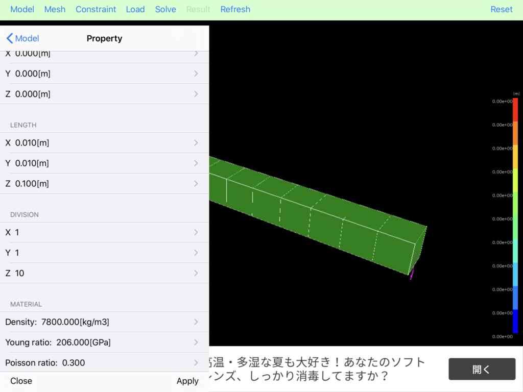
Modify the size of the model
When you launch the app, the cantilever beam is already available as an example model. Since the default shape is 0.1m x 0.1m x 1m, modify the dimensions as the above example. Note that the length unit in the app is [m].
On the App screen, from the menu, select “Model” -> “Rect1” -> LENGTH and correct X and Y to 0.01 [m] and Z to 0.1 [m].
Tap the “>” at the right end of each Table item, and the picker view will appear, so enter the value.
After entering the value, tap “Apply” at the bottom right of the Property view.
Note that the changes will not be reflected unless “Apply” is tapped.
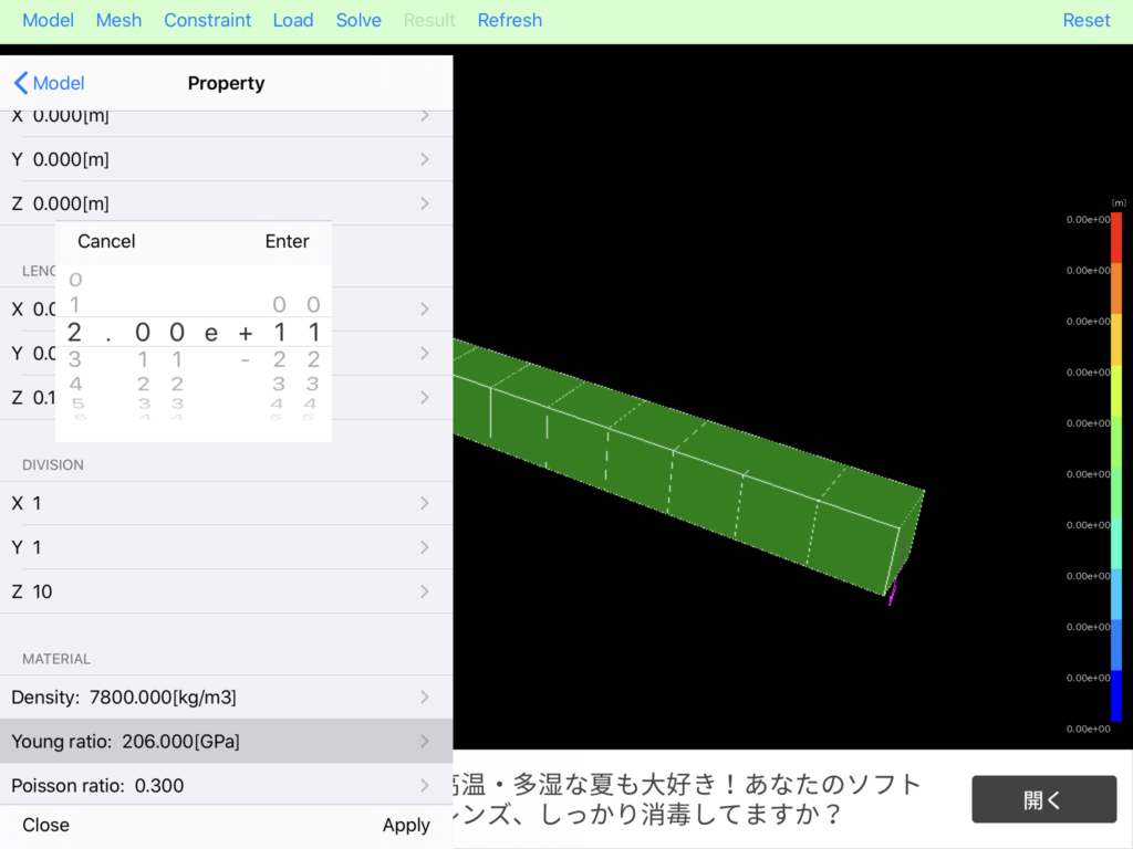
Set the material values
By default, the app contains the material values for general steel. Modify the Young’s modulus from the default value of 206GPa to the example of 200GPa.
From the menu, select “Model” -> “Rect1” -> MATELIAL Young ratio
Since it is 200 GPa, enter 2.00 e+11.
Don’t forget “Apply” here as well.
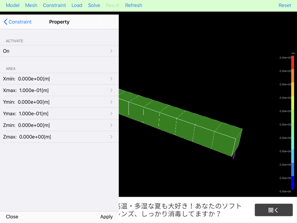
Check the boundary condition
Boundary conditions with one end fixed are created when the application is launched, but please check it.
From the menu, select “Constraint” -> “Constraint 0”.
The nodes in the range set by AREA are fixed
In AREA, the range of the leftmost face of the beam is automatically entered.
Make sure that ACTIVATE is On and close the table.
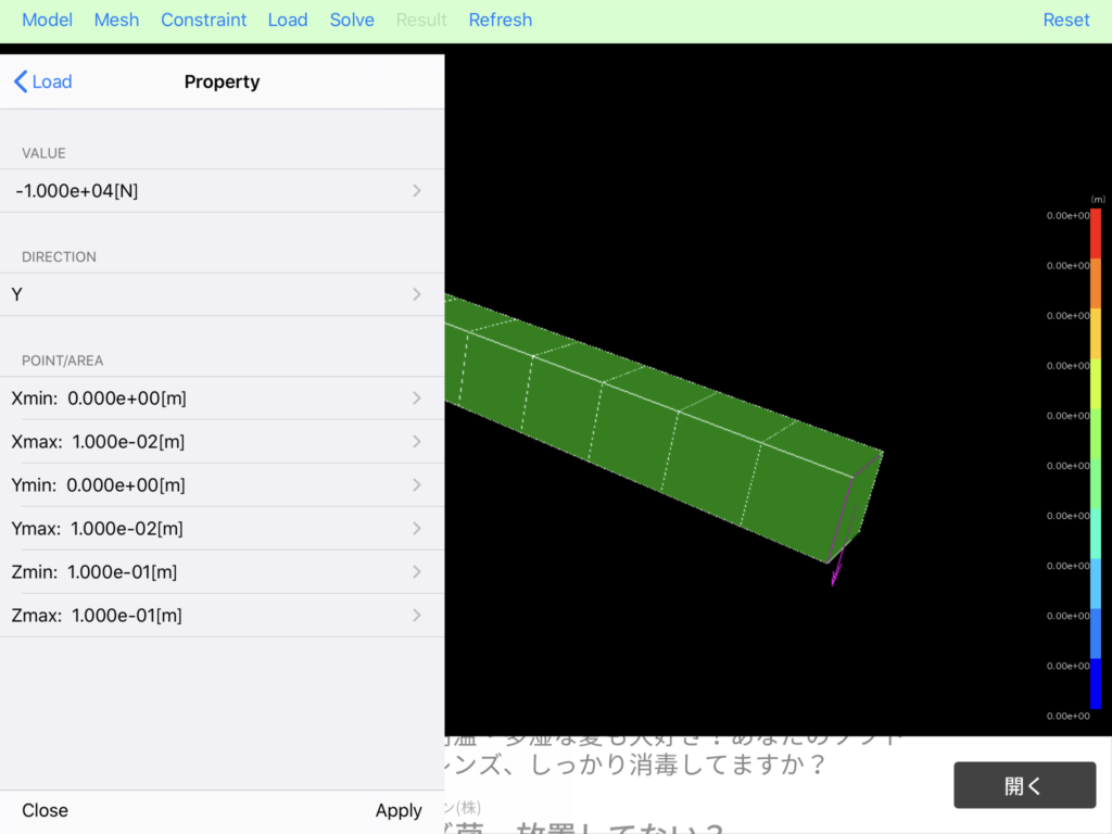
Modify the external force
External force is also set in advance in the bending direction on the free end. Modify the magnitude of the load according to the example. Also, since the dimensions have been changed, the range of the free end need also be modified.
From the menu, select “Load” -> “Load 1” .
Modify VALUE to “-1.0 e+04”.
At POINT/AREA, modify Xmax to 1.0e-02, Ymax to 1.0e-02, Zmin to 1.0e-01 and Zmax to 1.0e-01.
Tap “Apply”.
Execute the linear static analysis
Now the analysis is ready. Execute the static analysis.
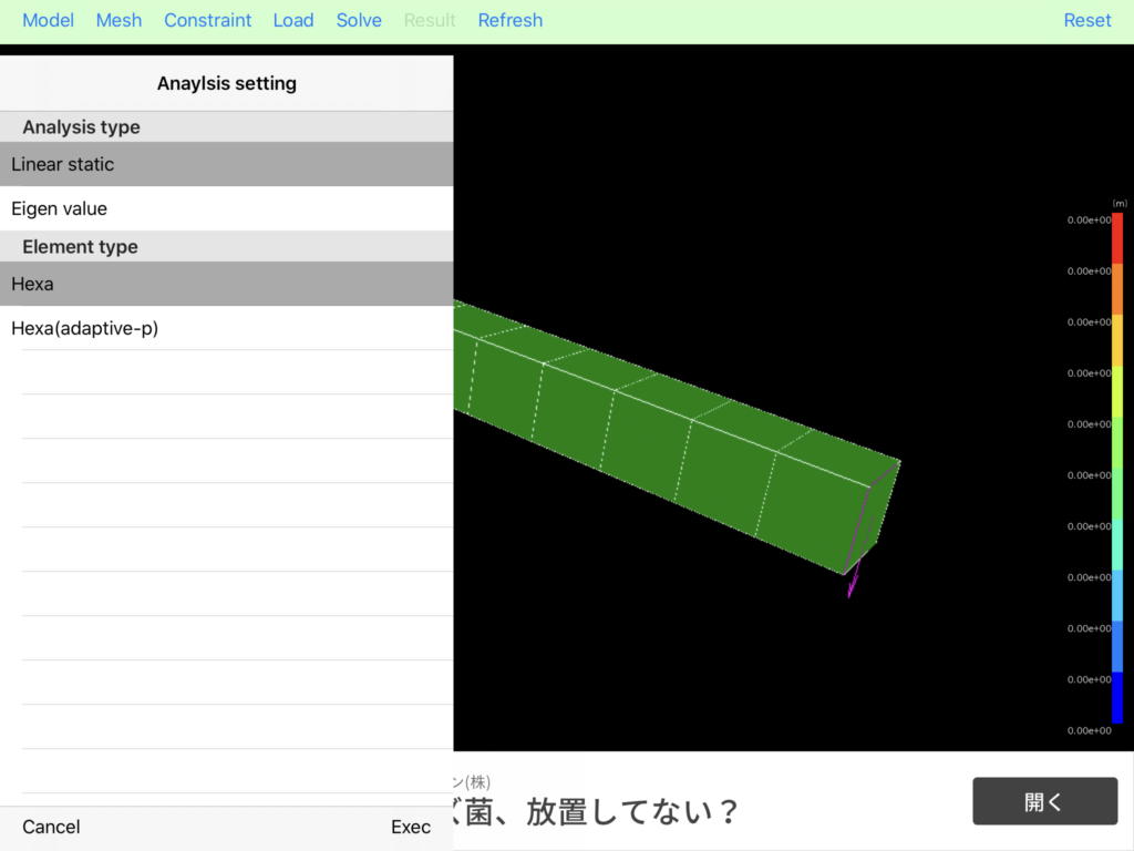
From the menu, tap “Solve”. Analysis Setting view will be appeared.
Confirm that “Linear static” is selected in Analysis type.
Make sure “Hexa” is selected for Element type.
Tap “Exec” at the bottom right.
Since it is a small model, analysis can be completed in an instant.
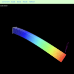
See the results
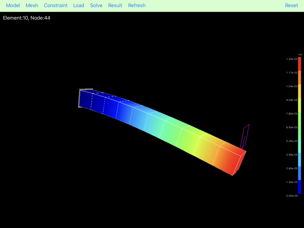
Although the current App only gives a rough result, it is sufficient for this example to obtain the maximum displacement at the free end. The value at the top of the contour bar(at the right end of the App screen) means the maximum displacement value. Probably it is “1.30e-02”. That is 0.013 [m].
The theoretical solution is 0.02[m] from the above example article. See Figure 5 in the article. Although we used different type of the element, it seems that the result is almost the same as the division number 1 of CFEM-SHELLr.
Modify the mesh and execute the analysis again
Now, let’s increase the number of divisions until sufficient accuracy is obtained, similar to the general FEM analysis procedure. Adjusting the mesh size is an important process of FE analysis. Let’s do it with this App.
If the result is displayed, tap “Delete” at the bottom right of the menu “Result”. The model will return to the green state.
Here, according to the example article, I would like to modify the number of divisions.
・Menu “Model” -> “Rect1” -> DIVISION
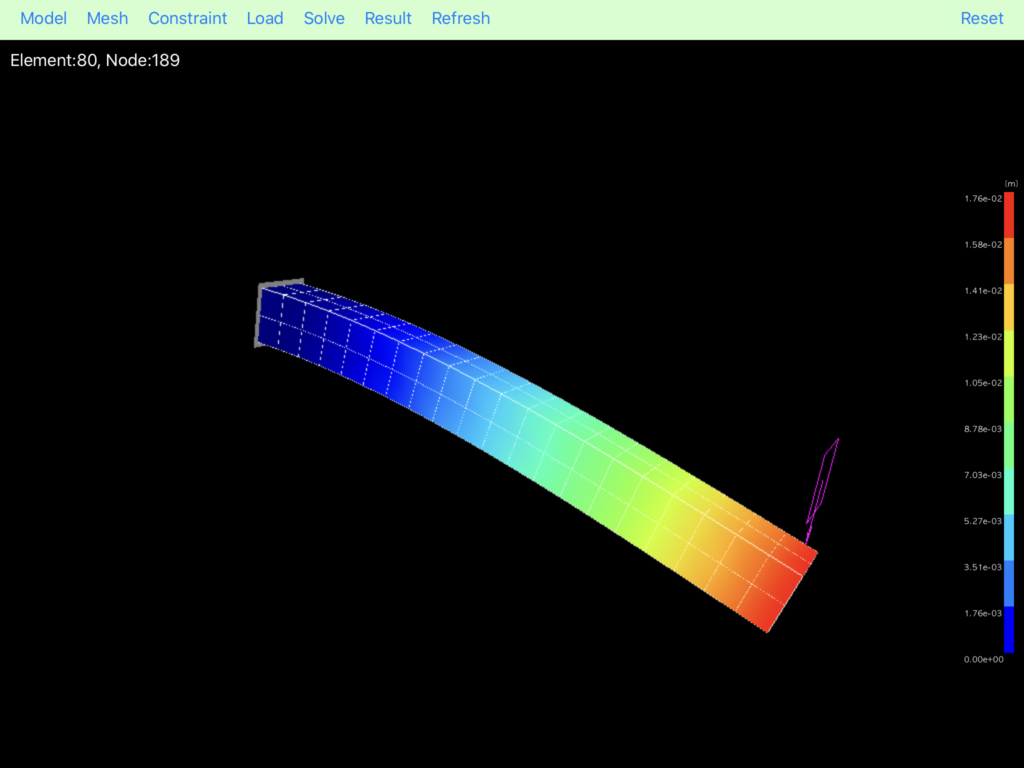
Changed from X:1, Y:1, Z:10 to X:2, Y:2, Z:20
・Execute the static analysis as before.
・If “You need to see the rewarded video” is displayed, press OK to see the advertisement, and then analysis will be performed. The advertisement is Admob provided by Google. This flow is as a free App, so there is no help for it.
・Confirm the maximum displacement in the result.
・Increase the number of divisions until the maximum displacement becomes approximately 0.02 [m].
* To change the mesh size uniformly, from the menu “Mesh”, tap “>” at the right end of Mesh sizes and enter the value in the picker view.
Summarize the results
Number of division Max displacement[m]
1 x 1 x 10 0.013
2 x 2 x 20 0.0176
4 x 4 x 40 0.0194
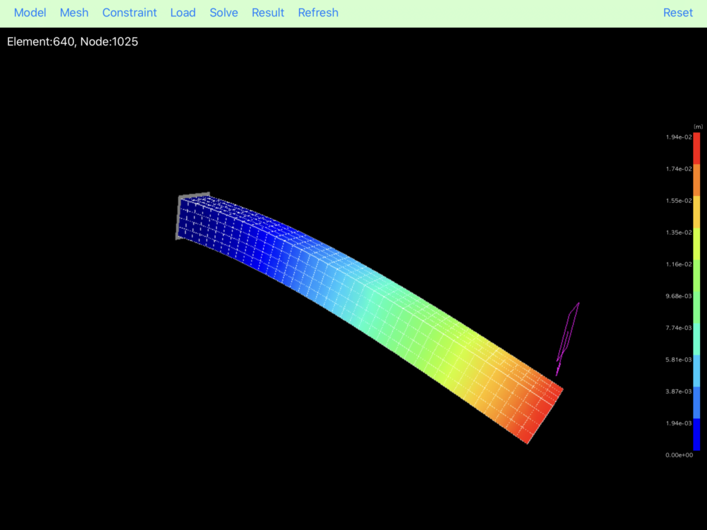
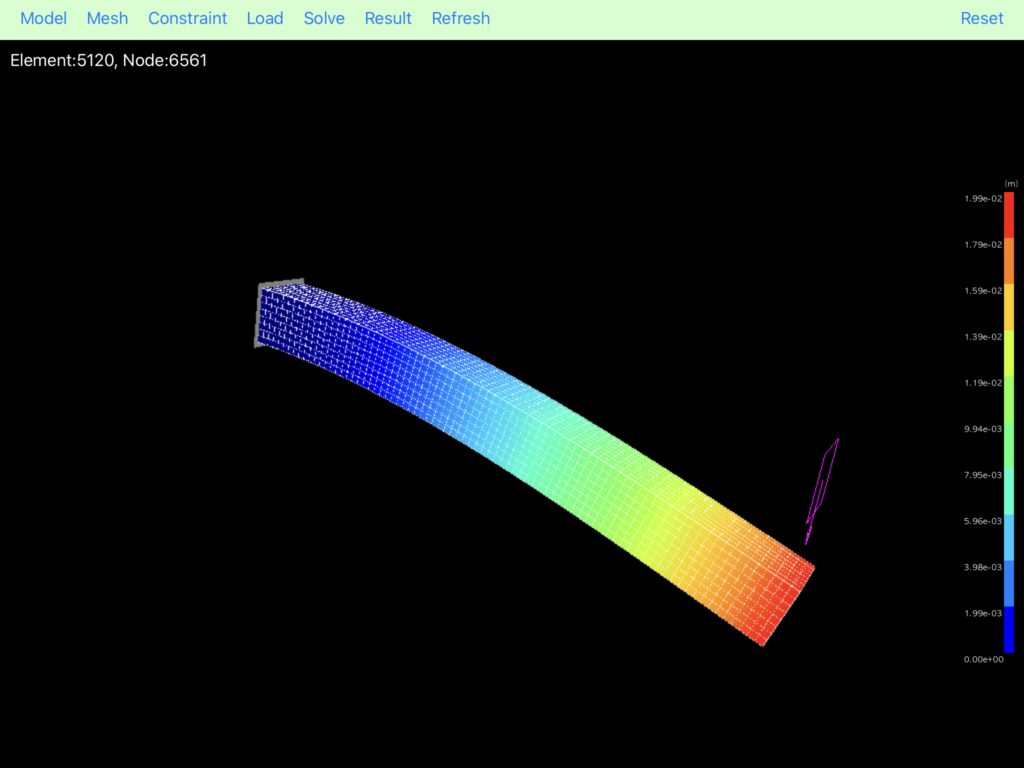
8 x 8 x 80 0.0199
(Note that the maximum number of elements of this application is 20,000)
With 8x8x80 division, it almost matches with the theoretical solution. It is the same tendency as the example article. Even with this App, the basic analysis “static analysis of a cantilever” can be sufficient.
Demo video (YouTube)
That’s all…